Tutorial 2 Niche query benchmark on DLPFC dataset

To systematically benchmark niche querying performance on real datasets with a substantial number of samples, we used the Human Dorsolateral Prefrontal Cortex32 (DLPFC) dataset. This dataset consists of 12 well-annotated spatial transcriptomic samples with a total of types of layers.

import os
os.environ['CUDA_VISIBLE_DEVICES'] = '0'
import sys
import logging
import warnings
import numpy as np
import scanpy as sc
import matplotlib.pyplot as plt

import sys, os
import quest.utils as utils
from quest.trainer import QueSTTrainer

warnings.filterwarnings("ignore")
logger = logging.getLogger(__name__)
logging.basicConfig(level=logging.WARNING)

Read and explore the data

data_path = "../data/DLPFC"
model_path = "../results/DLPFC/model/quest_model.pth"
sample_ids = ["151507", "151508", "151509", "151510", "151669", "151670",
              "151671", "151672", "151673", "151674", "151675", "151676"]
adata_list = [sc.read_h5ad(f"{data_path}/{data_id}.h5ad") for data_id in sample_ids]

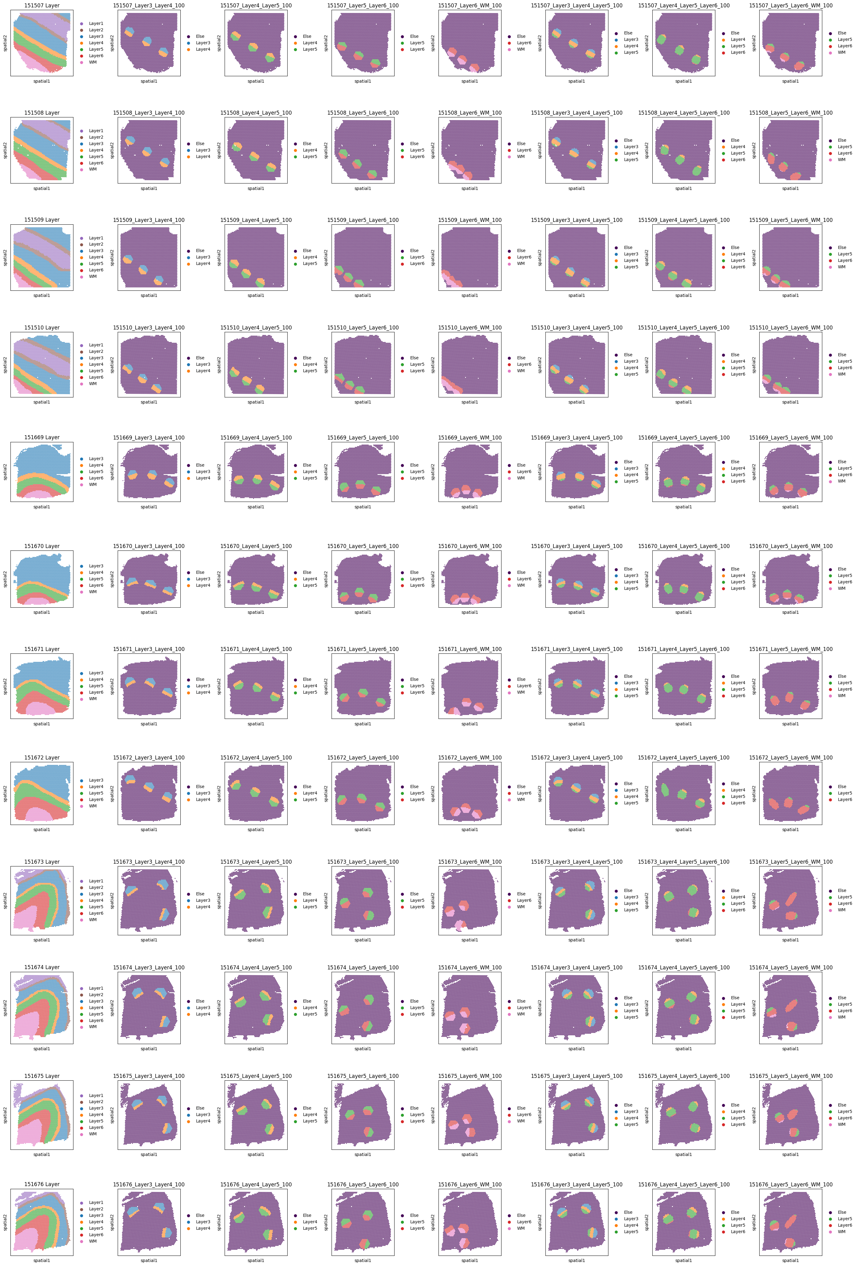
To include various layer composition scenarios, we defined seven niche types: four composed of two layers, and the rest three composed of three layers. For each niche type, we randomly sampled three replicates in each sample.

niche_groups = ["Layer3_Layer4_100", "Layer4_Layer5_100", "Layer5_Layer6_100", "Layer6_WM_100",
                "Layer3_Layer4_Layer5_100", "Layer4_Layer5_Layer6_100", "Layer5_Layer6_WM_100"]
niche_replicates = [0, 1, 2]

Here we show all the query niches and ground truth layer annotation.

nrows, ncols = 12, 8
fig, axs = plt.subplots(nrows, ncols, figsize=(28, 42))  # figsize is (col, row)
axs = axs.flatten()
for i, sample_name in enumerate(sample_ids):
    sc.pl.spatial(adata_list[i], color="Layer", ax=axs[i * ncols], spot_size=5, show=False, palette=utils.color_dlpfc, title=f"{sample_ids[i]} Layer")
    axs[i * ncols].invert_yaxis()
    for j, niche_group in enumerate(niche_groups):
        title = f"{sample_name}_{niche_group}"
        sc.pl.spatial(adata_list[i], color=f'{niche_group}_layer', spot_size=5, ax=axs[i * ncols + j + 1], show=False, palette=utils.color_dlpfc, title=title)
        axs[i * ncols + j + 1].invert_yaxis()
fig.tight_layout()
fig.show()

Configure niche query task

Here we use the niche named Layer5_Layer6_100_replicate=0 on sample 151670 as an example.

dataset = "DLPFC"
query_sample_id = "151670"
query_niches = ['Layer5_Layer6_100_replicate=0_niche']

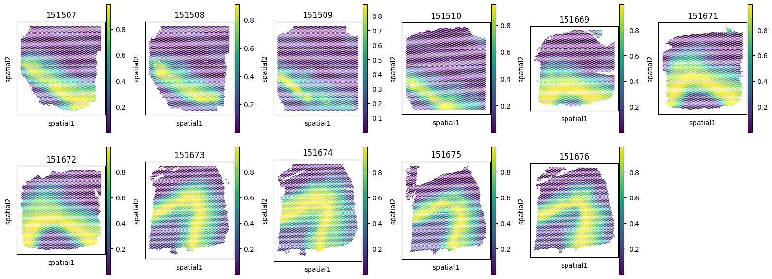
We also show the Region Matching Score of this query niche on the other referene samples. We use this score as a ground truth niche similarity measurement.

adata_ref_list = [adata for adata in adata_list if adata.uns['library_id'] != query_sample_id]
ref_id_list = [adata.uns['library_id'] for adata in adata_ref_list]
adata_plot = adata_list[sample_ids.index("151673")]
fig, axes = plt.subplots(ncols=6, nrows=2, figsize=(16, 6))
axes = axes.flatten()
for i, adata_ref in enumerate(adata_ref_list):
    sc.pl.spatial(adata_ref, color=f"{query_sample_id}_Layer5_Layer6_100_replicate=0_region_matching_score",
                  spot_size=5, show=False, title=f"{adata_ref.uns['library_id']}", ax=axes[i])
    axes[i].invert_yaxis()
axes[11].axis('off')
fig.suptitle(f"Region Matching Score of Query niche: {query_niches[0]} on {query_sample_id}")
fig.tight_layout()
fig.show()

Set up QueST Trainer

trainer = QueSTTrainer(dataset=dataset, data_path=data_path, sample_ids=sample_ids, adata_list=adata_list,
                       query_niches=query_niches, query_sample_id=query_sample_id,
                       model_path=model_path,
                       epochs=20, save_model=True, hvg=4000, min_count=0, normalize=True, seed=2024)

Train QueST model and perform niche query

We also provided pretrained QueST model checkpoint weights at https://cloud.tsinghua.edu.cn/d/d0497bcee4e34a76aaf8/. To skip training and use pretrained checkpoint, simiply put it at corresponding model path and comment the “trainer.train()” line.

trainer.train()
trainer.inference(ckpt_path=model_path, save_embedding=False, query=True)

computing 3-hop subgraph (151507): 100%|██████████| 4221/4221 [00:05<00:00, 766.92it/s]
computing 3-hop subgraph (151508): 100%|██████████| 4381/4381 [00:05<00:00, 801.77it/s]
computing 3-hop subgraph (151509): 100%|██████████| 4788/4788 [00:05<00:00, 799.55it/s]
computing 3-hop subgraph (151510): 100%|██████████| 4595/4595 [00:05<00:00, 792.83it/s]
computing 3-hop subgraph (151669): 100%|██████████| 3636/3636 [00:04<00:00, 794.55it/s]
computing 3-hop subgraph (151670): 100%|██████████| 3484/3484 [00:04<00:00, 793.57it/s]
computing 3-hop subgraph (151671): 100%|██████████| 4093/4093 [00:05<00:00, 793.95it/s]
computing 3-hop subgraph (151672): 100%|██████████| 3888/3888 [00:04<00:00, 793.61it/s]
computing 3-hop subgraph (151673): 100%|██████████| 3611/3611 [00:04<00:00, 800.92it/s]
computing 3-hop subgraph (151674): 100%|██████████| 3635/3635 [00:04<00:00, 793.74it/s]
computing 3-hop subgraph (151675): 100%|██████████| 3566/3566 [00:04<00:00, 792.50it/s]
computing 3-hop subgraph (151676): 100%|██████████| 3431/3431 [00:05<00:00, 680.86it/s]
training: 100%|██████████| 20/20 [13:27<00:00, 40.35s/epoch]

fig, axes = plt.subplots(ncols=6, nrows=2, figsize=(16, 6))
axes = axes.flatten()
query_niche = query_niches[0]
adata_ref = trainer.adata_ref_list[0]
for i, adata_ref in enumerate(trainer.adata_ref_list):
    sc.pl.spatial(adata_ref, color=f"{query_niche} predicted matching score", ax=axes[i], show=False,
                  spot_size=5, title=f"{adata_ref.uns['library_id']}")
    axes[i].invert_yaxis()
axes[11].axis('off')
fig.tight_layout()
fig.show()